Introduction

Deep generative models for graphs have shown great promise in the area of drug design, but have so far found little application beyond generating graph-structured molecules. In this work, we demonstrate a proof of concept for the challenging task of road network extraction from image data introducing the Generative Graph Transformer (GGT): a deep autoregressive model based on state-of-the-art attention mechanisms. In road network extraction, the goal is to learn to reconstruct graphs representing the road networks pictured in satellite images. A PyTorch implementation of GGT is available here.

Methods

The proposed GGT model is designed for the recurrent generation of graphs, conditioned on other data such as an image, by means of the encoder-decoder architecture outlined in Fig. 1. Although in our experiments the model is specific to image-conditioning, the encoder could be easily changed to have a generation conditioned on graphs, text, feature vectors, or not conditioned at all.

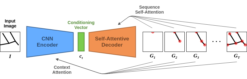
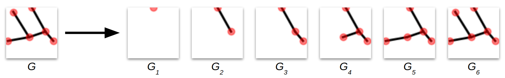
In the image-conditioned generation, the encoder takes as input an image \(\mathbf{I} \in \mathbb{R}^{64\times 64}\) and emits a conditioning vector \(\mathbf{c} \in \mathbb{R}^{900}\), a compressed representation of the original input. The decoder takes as input the conditioning vector \(\mathbf{c}\) and recurrently generates the graph \(\mathcal{G} = \big(\tilde{\mathbf{A}} \in \mathbb{R}^{N \times N}, \tilde{\mathbf{X}} \in \mathbb{R}^{N \times 2}\big)\) through a sequence of node and edge additions starting from the empty graph. To learn the generative process, we take inspiration from You et al. (2018) and use a canonical ordering based on BFS. In our blog post introducing the Toulouse Road Network dataset, which we use to benchmark the GGT, we explain in details how the canonical ordering for the graphs is generated. In Fig. 2 we plot an example of canonical ordering for a graph based on the BFS.

Decoder

The decoder network in the GGT is based on transformer networks firstly introduced by Vaswani et al. (2017). In Fig. 3 we present a schema of the decoder, labeling the main components.

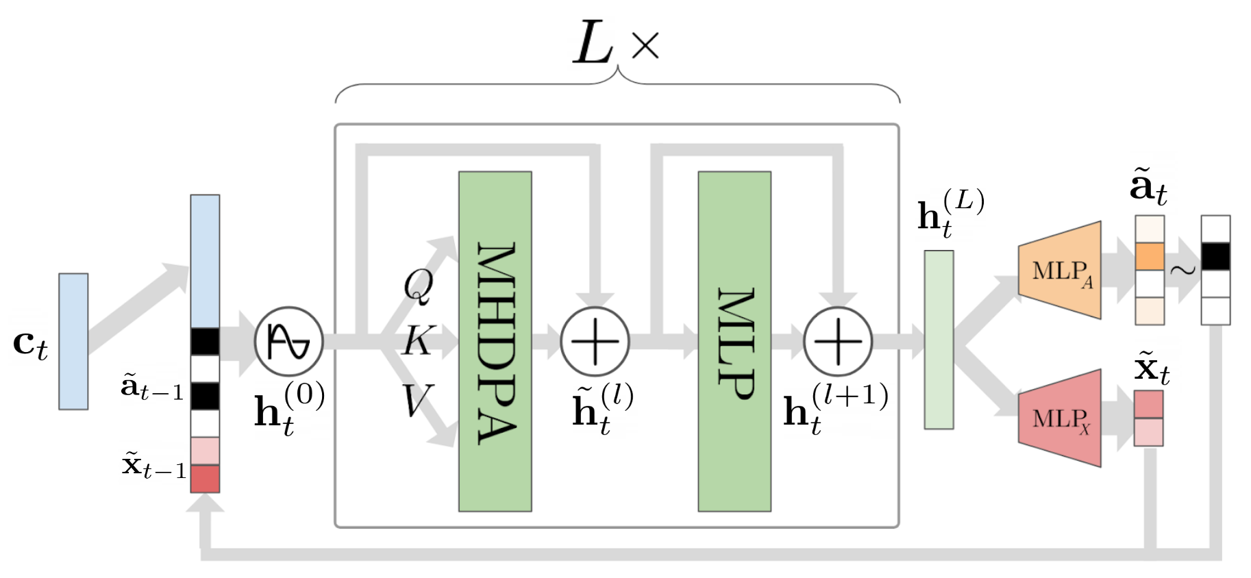
At every time-step \(t\) in the recurrent genreation, the decoder takes as input the conditioning vector \(\mathbf{c}\) and the representation of the last node generated in the sequence, described by its adjacency vector \( \tilde{\mathbf{a}}_{t-1}\) and node coordinates \( \tilde{\mathbf{x}}_{t-1}\). First, the concatenated inputs are positionally encoded and passed through a linear layer to obtain the first hidden representation of the current graph \[\mathbf{h}_{t}^{(0)} = \mathbf{W}_{in} \big(\big[\tilde{\mathbf{a}}_{t-1}, \tilde{\mathbf{x}}_{t-1}, \mathbf{c}_t \big] + \mathbf{p}_t\big) \in \mathbb{R}^d,\] where \(d=256\). Next, as in the original transformer networks, a sequence of \(L\times \) decoding blocks transform the representation of the graph as in: \[\tilde{\mathbf{h}}_t^{(l)} = \operatorname{LN}\big(\mathbf{h}_t^{(l)} + \operatorname{MultiHead}(\mathbf{h}_t^{(l)},\mathbf{h}_{< t}^{(l)})\big)\] and \[\mathbf{h}_t^{(l+1)} = \operatorname{LN}\big(\tilde{\mathbf{h}}_t^{(l)} + \mathbf{W}_n^{(l)}\operatorname{ReLU}(\mathbf{W}_m^{(l)}\tilde{\mathbf{h}}_t^{(l)})\big), \] finally obtaining the last hidden representation \(\mathbf{h}_t^{(L)}\). In these equations, the MultiHead operator refers to the self-attention as in Vaswani et al. (2017), LN is layer normalization (Ba et al., 2017), and \( \forall l, \quad \mathbf{W}_m^{(l)} \in \mathbb{R}^{2048\times d}\), \(\mathbf{W}_n^{(l)} \in \mathbb{R}^{d\times2048}\), \(\mathbf{h}_t^{(l)}, \tilde{\mathbf{h}}_t^{(l)} \in \mathbb{R}^d\). Following, two MLP heads are responsible for the emission of the node coordinates and adjacency vector representing the next node in the graph. Formally, they are defined as: \[ \tilde{\mathbf{x}}_t = \operatorname{tanh} \big( \mathbf{W}_{x2} \operatorname{ReLU}(\mathbf{W}_{x1} \mathbf{h}_t^{(L)})\big), \] \[ \tilde{\mathbf{a}}_t = \sigma \big( \mathbf{W}_{a2} \operatorname{ReLU}(\mathbf{W}_{a1} \mathbf{h}_t^{(L)})\big), \] where \(\mathbf{W}_{a1}, \mathbf{W}_{x1} \in \mathbb{R}^{128\times d}\), \(\mathbf{W}_{a2} \in \mathbb{R}^{M\times128}\), \(\mathbf{W}_{x2} \in \mathbb{R}^{2\times128}\), and \(M\) is the maximum size of the frontier in the BFS-ordering. The soft adjacency vector \(\tilde{\mathbf{a}}_t\) can be sampled or thresholded to obtain a binary vector.

Encoder

To condition the generative process, we use a simple CNN encoder which takes as input a semantic segmentation \(\mathbf{I} \in \mathbb{R}^{64\times 64}\) and emits a low-dimensional representation as \(\mathbf{c} = \operatorname{CNN}(\mathbf{I}) \in \mathbb{R}^{900}\). Furthermore, we introduce an image attention mechanism on the CNN encoder based on the context attention proposed by Xu et al. (2015), which we outline in Fig. 4.

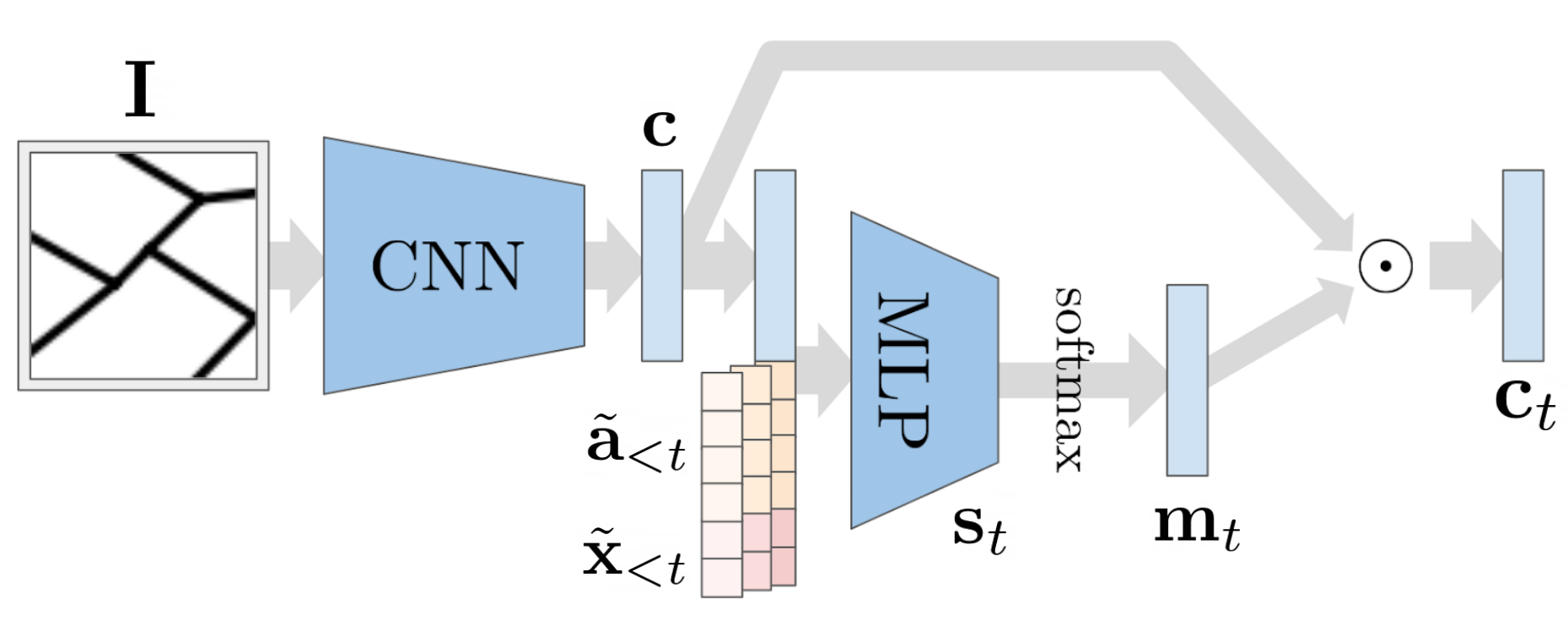
This mechanism is implemented as an MLP which takes as input the flattened visual features \(\mathbf{c}\) and the previously generated node features \(\tilde{\mathbf{x}}_{ %lt t }\) and \(\tilde{\mathbf{a}}_{ %lt t }\), and outputs a mask vector: \[ \mathbf{s}_t = \mathbf{W}_{c2} \operatorname{ReLU}(\mathbf{W}_{c1} [\tilde{\mathbf{a}}_{< t}, \tilde{\mathbf{x}}_{< t}, \mathbf{c}]),\] \[ \mathbf{m}_t = \frac{\operatorname{exp}(\mathbf{s}_t)}{\sum_{i=1}^{|\mathbf{s}_t|} \operatorname{exp}({{\mathbf{s}}_t}_i)},\] \[ \mathbf{c_{t}} = \mathbf{{c}} \odot \mathbf{m}_t,\] where \({\mathbf{W}}_{c1}, {\mathbf{W}}_{c2}^\top \in \mathbb{R}^{1800\times 900}\), \(\mathbf{s}_t\) is the vector of attention scores of length \(|\mathbf{s}_t|=900\), and \(\mathbf{m}_t\) is the mask vector applied on the visual features through the element-wise product operation \(\odot\).

Training setup

To train the GGT we use a loss function which combines two components determining the quality of the generated graph: \[ \mathcal{L} \,\,= \,\, \lambda \mathcal{L}_{\mathbf{A}} + (1-\lambda) \mathcal{L}_{\mathbf{X}} \,\,=\,\, \lambda \operatorname{BCE}(\tilde{\mathbf{A}}, \mathbf{A}) + (1-\lambda) \operatorname{MSE}(\tilde{\mathbf{X}}, \mathbf{X})\] The Binary Cross Entropy between the target and predicted adjacency matrices captures the structural error, while the Mean Squared Error between target and predicted node coordinates captures the error in the position of the nodes. The hyperparameter \(\lambda\) regulates the tradeoff between the two loss components. The model is trained using teacher forcing. \( \)

Evaluation Metrics

To evaluate and compare the different models we need to choose a suitable metric. In particular, an effective evaluation metric should be able to capture the quality of reconstructed graphs while being independent from the ordering used to learn the generative process. Indeed, the generated graph may have additional or missing nodes while still describing accurately the road network. Moreover, we would like a metric to be invariant to graph transformations and node permutations, and efficient to compute. Since commonly used metrics do not satisfy these properties, we introduce a new evaluation metric based on an approximation of the earth mover's distance which we call StreetMover distance. In Fig. 5 we sketch the steps taken to compute the StreetMover distance between a predicted and target graph.

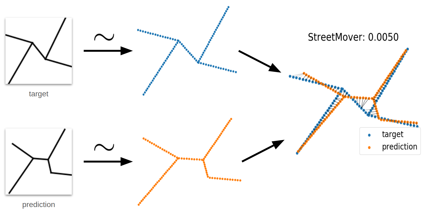
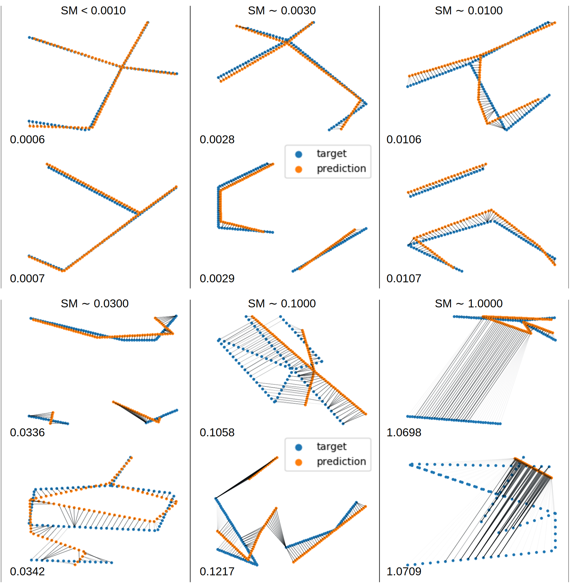
To compute the Streetmover distance, we first approximate each graph by sampling equidistantly over the edges a 2D point cloud with a fixed number of points. Afterwards, we approximate with the Sinkhorn distance (Cuturi, 2013) the computation of the optimal transport cost between the two point clouds by means. This distance can be efficiently computed using Sinkhorn iterations, which makes it a better candidate with respect to Wasserstein distance. By plotting the coupling matrix between the point clouds we can visually interpret the cost of moving streets or part of them to perfectly match the target road network. In Fig. 6 we visualize the Streetmover distance for different samples of target and predicted graphs. We see how our metric is effective in capturing the quality of the reconstructions, with the distance value being closely related to the accuracy of the reconstructed graphs.

An alternative evaluation metric for road network comparison is the Average Path Length Similarity, introduced in . However, we choose not to use APLS as it requires some significant post-processing and it is mainly designed to capture errors in semantic segmentations of road networks rather than their graph representation. To support the scores obtained in terms of Streetmover distance, we also report additional evaluation metrics, like validation loss, average error in the number of nodes \(|V|\) and edges \(|E|\), and Wasserstein distance between histogram of node degree and diameters of the connected components.

Experimental Results

We run a set of experiments comparing the performance of GGT with several baseline models on the task of Road Network Extraction. The baseline models use the following decoder networks: a simple MLP, a simple GRU, GraphRNN extended for labeled graph generation, GRU and GraphRNN with self-attention. More details regarding the baselines are presented in the paper. The same hyper-parameter search is performed for all the model using a validation set.

Quantitative Results

In Table 1 we compare the performance of the Generative Graph Transformer with various baselines for the task of Road Network Extraction.

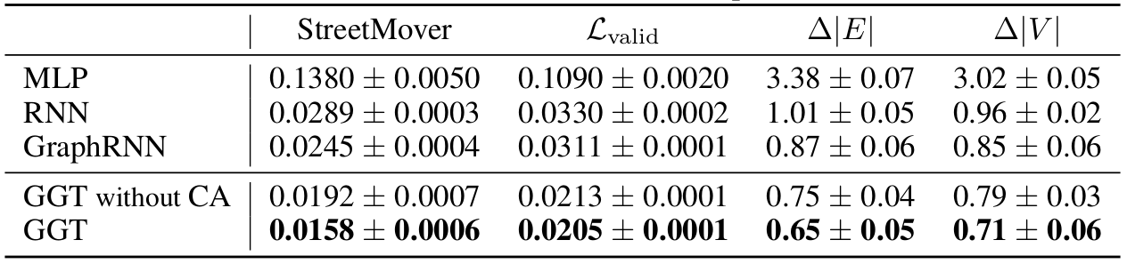
We notice how the simplest model with MLP decoder completely fails in reconstructing road network, while the recurrent generation of graphs through GRU and GraphRNN decoders seems more effective. Simple self-attentionmechanisms further improve the scores for the considered metrics. The best results are obtained with the Generative Graph Transformer decoder, especially when paired introducing context attention (CA) in the encoder. In this evaluation we set \( \lambda = 0.5 \). In further experiments reported in the paper, we explore the effect of changing this hyperparameter, and find the optimal values to be in the range \( [0.3, 0.7] \).

Qualitative Results

To validate the observations drawn from the quantitative study, we further validate the results through a set of qualitative studies.

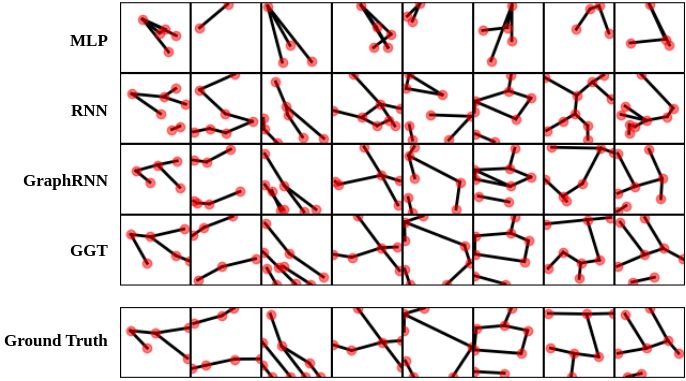
We first compare, in Fig. 7, the reconstruction of road networks randomly drawn from the test set using different models. The difference in accuracy among difference models is evident and in line with the previous numerical observations.

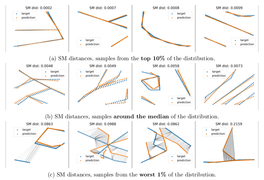
In Fig. 8 we only consider the Generative Graph Transformer and plot exampels of the best, median and worst reconstructions in the test set according to StreetMover distance. Graphs in the top 10% are reconstructed almost perfectly, and are mostly simpe graphs with few edges and low branching factor. Graphs around the median of the StreetMover distance also have accurate reconstructions, with minor noise in the node coordinates. We see graphs with more complex structures like loops, high number of edges and branches, and many connnected components. Looking at some bad reconstruction, drawn from the bottom 1% of the test set, we witness two types of failure from the model. In the first case, the model is generating some additional component which is not present in the original road network, or it is missing to generate some components from the ground-truth. In the second case, the model is completely failing to generate a meaningful graph. We notice that in this case the coordinates of the first emitted node are completely wrong, and this results in divergence in the generation of the rest of the BFS-ordered seqence of nodes. We hypotehsize, and leave it as future work, that more sophisticates sampling techniques like beam search would significanly reduce this type of failure.

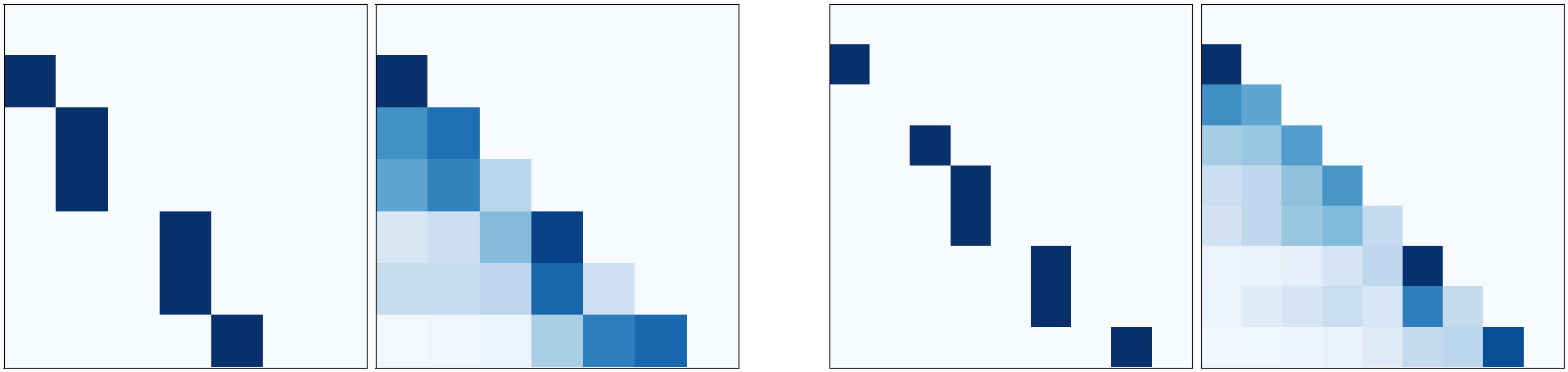
By inspecting the self-attention layers in the GGT, we see in Fig. 9 how some heads are responsible for learning the structure in the graphs, emitting attention weights that highly correlate with the corresponding lower triangular adjacency matrices (lower triangular matrices are plotted because of the future masking in the self-attentive generation).

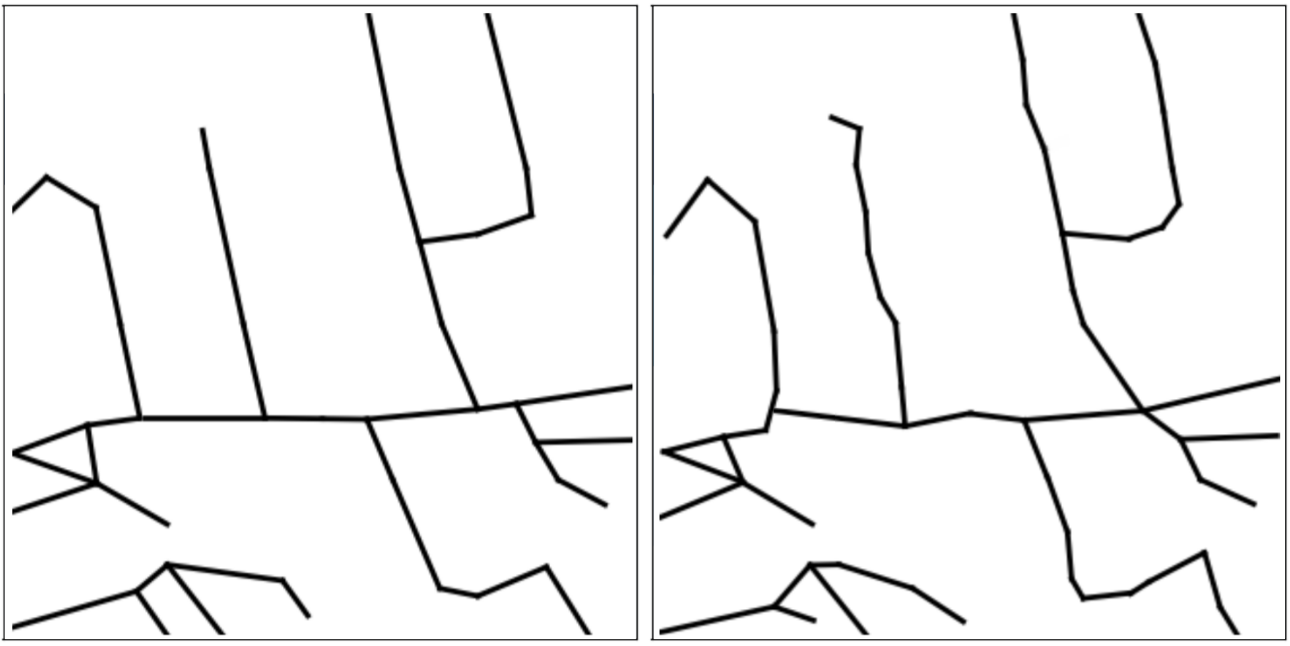
Finally, in Fig. 10, we show how graphs from adjacent patches can be easily merged to reconstruct road networks at larger scales. For this experiment we randomly select a 4x4 grid of datapoints in the test region and reconstruct the road networks using the GGT. We then use a simple post-processing step to join together closeby nodes laying in the borders of two consecutive patches. Although a very naive approach is used to merge together multiple graphs the structure of the larger region is modeled accurately.

Conclusion and Future Work

In this post we presented the Generative Graph Transformer, a deep autoregressive model based on self-attention for the recurrent, conditional generation of graphs. Moreover, we introduced the StreetMover distance, a scalable, efficient and permutation-invariant metric for graph comparison. We benchmarked the GGT for the task of road network extraction starting from segmentations of satellite images, comparing the results with many baselines. A challenge that remains open in this field is the development of a complete end-to-end solution combining semantic segmentation and graph extraction. Applying the proposed GGT model to other graph generation tasks, such as drug design, is another interesting direction for future work.