Introduction

This blog post presents the Toulouse Road Network dataset, firstly introduced in Belli and Kipf (2019). This dataset is proposed to benchmark models in the task of image-conditioned graph generation, specifically for road network extraction from segmentations of satellite image data. The Python code to generate the dataset, the PyTorch interface for its usage as well as the instructions to download the ready-to-use dataset are available here.

In the general task of road network extraction the inputs are raw satellite images and the target is to reconstruct the underlying graph representation of the network. However, most recent approaches (Muruganandham, 2016; Henry et al., 2018; Etten et al., 2018; Gao et al., 2019; Gao et al., 2019) are limited to the generation of semantic segmentation of road networks, possibly using hand-engineered post-processing steps and heuristics to finally extract a graph representation. In our work, we try to bridge this gap by introducing an automated, fully differentiable model which generates graph representations from semantic segmentations. We discuss the proposed model in another blog post introducing the Generative Graph Transformer.

Dataset Generation

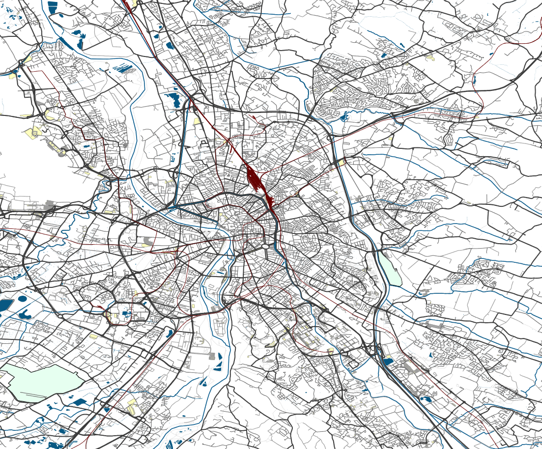
To generate the Toulouse Road Network dataset we start from publicly available raw data released by OpenStreetMap. OpenStreetMap is one of the biggest open-source web-applications for retrieving, reasoning and updating road maps and satellite data. In particular, GeoFabrik publicly released a few datasets of cities containing geographical information like railways, road networks, buildings, waterways in shapefile format. To introduce a dataset for image-to-graph generation, we extract, process and label the raw road network data from the city of Toulouse, France, available on GeoFabrik and time-stamped June 2017. Fig. 1 shows the streets, railways, waterways contained in the shapefile data.

In the rest of the blog post, we discuss a sequence of pre-processing and filtering steps designed to convert the raw data provided in shapefile format to explicit graph structures. Further, we extract the road map dataset as image and graph pairs, define train, validation and test splits, and briefly present some statistics of the dataset. Finally, we present our approach to extract unique orderings over the graph components by fixing a canonical ordering based on node-wise BFS-ordering. For more detailed information on the dataset extraction and PyTorch interface we redirect the reader to the documentation in the GitHub repository.

Preprocessing

In the source data, each road in the map is described as a sequence of line segments, and intersection points between different roads are not modeled. In particular, the data represents over 1100 squared kilometers of urban and extraurban area, with over 62,000 roads and 361,000 segments. A first sequence of transformations is used to extract a graph representation from the road segments, introducing new nodes in case of intersection, removing duplicate nodes and edges and normalizing node coordinates in \( [-1, +1] \). Afterwards, the whole map is divided in a grid of squares with a side length of 0.001 degrees, corresponding to around 110 metres. Each square in the grid is a candidate datapoint.

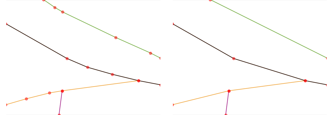
To remove noise in the graph representation to be learned by a deep learning model, we merge consecutive edges if the angle between them is close to \( \pi \), in particular where the incidence angle is between 75° and 90°. Furthermore, we merge together nodes if they are closer than \( {1 \over 20} \) the side of the square. In Fig. 2 we show an example of graph before and after the preprocessing. We use the same color for segments belonging to the same road in the original dataset.

Filtering

Taking a closer look at the graphs extracted until this point, we notice how a relevant percentage of the cells contain none or few segments of roads. We decide to filter the dataset generated so far by keeping only datapoints with at least 4 nodes in the graph. The reason motivating this filtering is that we consider trivial the automated extraction of simple graphs with less than 4 nodes from image representations. In addition to increasing the size of the dataset significantly and slowing the training process, it would be uninformative to test the capabilities of different generative models for such simple cases. We also remove the right tail of the graph distribution in terms of \(|V|\) and \(|E|\), in other words, outlier graphs with too many edges per image. These datapoints contain extremely cluttered and noisy graphs which are not informative and may harm the training process. The filtering of the right tail of the graph distribution is done at the 95th percentile of the distribution, removing graph with \(|V| \geq 10\) or \( |E| \geq 16\). At this point the graphs are plotted as grayscale \(64 \times 64\) semantic segmentations. In Fig. 3 we plot examples of road network segmentations extracted from the generated graph representations.

Augmentation

At this point, we augment the dataset using translation (shift), rotation and flipping. In particular, we translate the image (and the graphs) vertically and/or horizontally by \({1 \over 4}\) , \( {2 \over 4}\) or \( {3 \over 4}\) of the square side (augmentation factor \( \times 16\)). For rotations we use \({\pi \over 2}\) , \({ \pi}\) and \({3 \pi \over 2}\) angles, optionally flipping the source image (augmentation factor \(\times 8\) ). The total factor of augmentation is \( \times 128\) times the original number of datapoints. For limits in computational resources, the dataset we use in our experiments and release to the public only includes augmentation by translation.

Dataset splits

Finally, we split the datasets in training, valida- tion and test sets. To have consistent splits in terms of the distribution of datapoints, we use a row-column splitting criteria, as shown in Fig. 4.

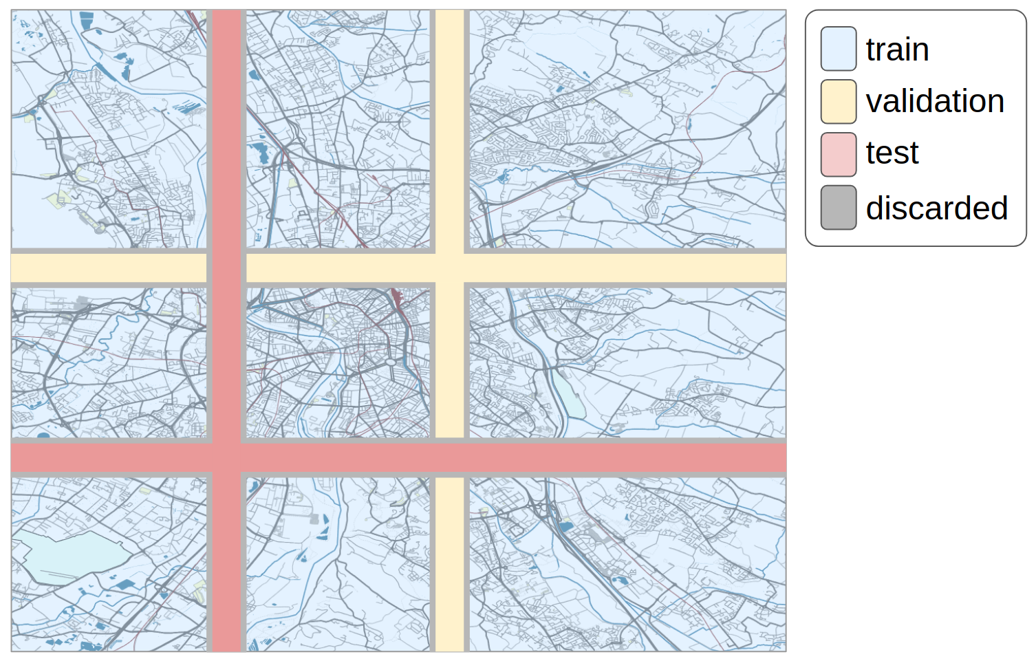
The idea of this splitting is that we want to capture similar distributions of graphs in each set. In Fig. 1 we saw how some areas of the map have very cluttered road networks, while others have sparse networks or no roads at all. The proposed way of splitting the dataset enforces enough diversity inside each split, and similarity between the distributions in dif- ferent splits. Since we are using translation in the augmentation, we also remove the regions of the grid at the edge between two different dataset splits, to avoid repetition of (part of) the graphs in different splits. This way of splitting the dataset also minimize the number of datapoints dis- carded in the conflict regions, and this is why we avoid random selection over the map to split the dataset.

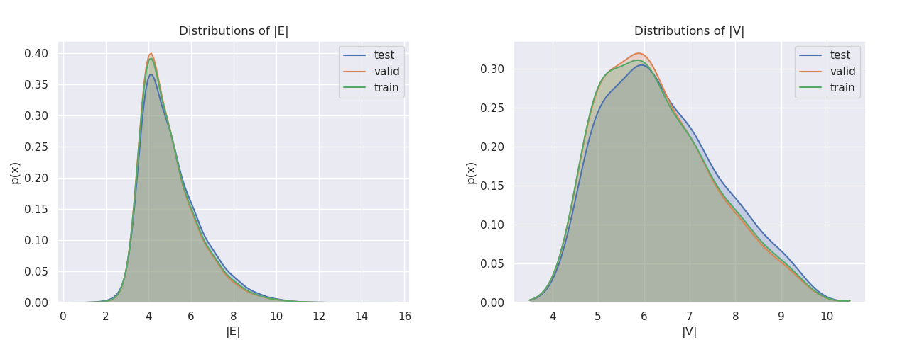
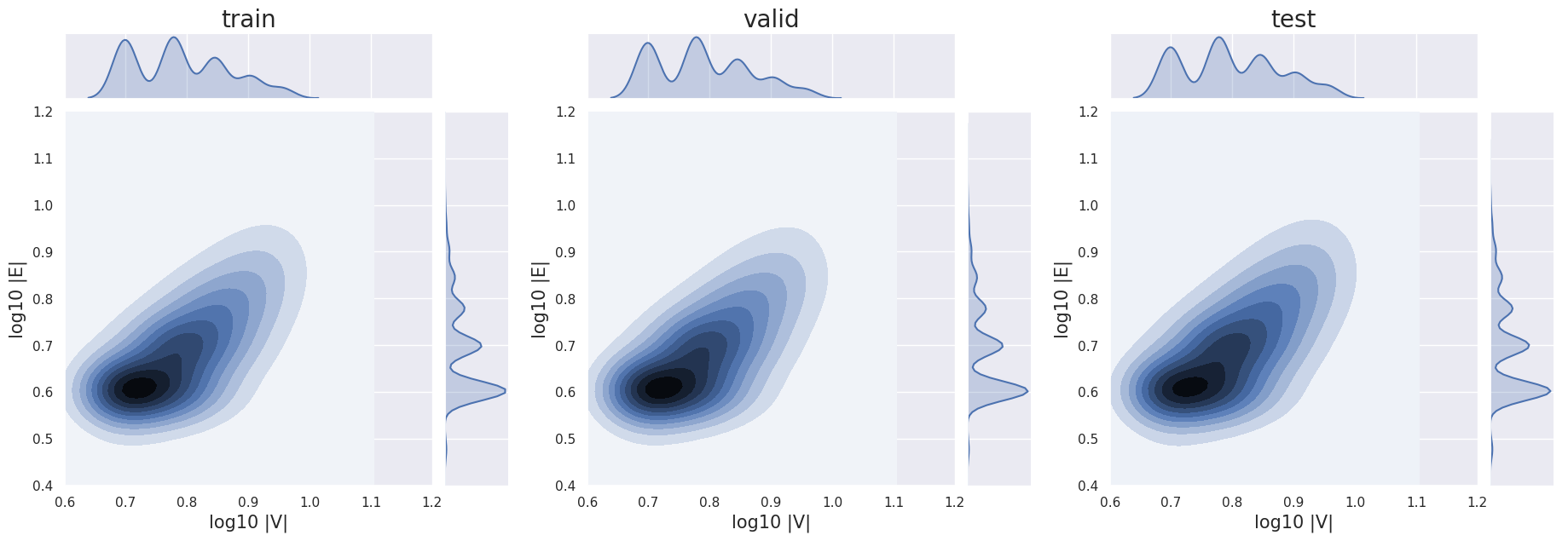
To ensure that the distribution of graphs in the training set is aligned with the ones in the validation and test set, we conduct a study on the marginal and joint distributions of |V | and |E| for different splits. In Fig. 5 we plot the marginal distributions of the datapoints in the three splits as a function of the number of nodes |V | in each graph and then we do the same as a function of the number of edges |E|. Furthermore, in Fig. 6 we compare the joint distributions of |V | and |E| for the three splits. We can see similar patterns in the marginal and joint distributions for different splits, confirming our hypothesis that the chosen criterium to split the dataset is effective in obtaining similar distributions in different splits.

The Toulouse Road Network dataset released with our splits contains 111,034 data points (map tiles), of which 80,357 are in the training set (around 72.4%), 11,679 in the validation set (around 10.5%), and 18,998 in the test set (around 17.1%).

Canonical Ordering

Each datapoint in our dataset is represented as a 64\(\times\)64 image and graph representation \(\mathbf{G} = (\mathbf{A}, \mathbf{X})\). However, since we are planning to generate the graph sequentially using a deep-autoregressive model, we need a linear representation of the road network.

For this, we take inspiration from You et al. (2018) and fix a canonical ordering on the graphs based on BFS-ordering over the nodes. Since we are working with planar graphs, we also need to choose a consistent way to break ties in the BFS happening in case of branches in a node and the appearence of multiple connected components. For this, we always start traversing a new connected component by choosing the top-left unvisited node in the graph. This includes the selection of the first node in the BFS. To break ties in case of branches in a node, we ordered the outcoming edges in that node clock-wise with respect to the direction of the incoming edge. 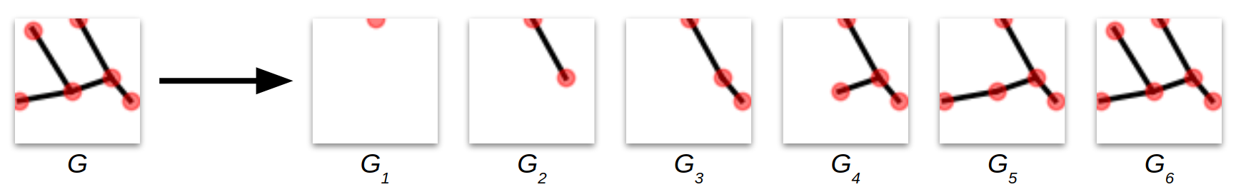In Fig. 7 we plot the linearization of a graph using the described canonical ordering, including the example of ties in the branching which occurs the second time-step in the BFS.

Conclusion

The Toulouse Road Network dataset is designed for future research aiming at automated systems for road network extraction, and more in general, to test deep learning models in the context of image-to-graph generation. Being large, customizable, and coming with an easy-to-use PyTorch Dataset API, it is a good option for benchmarking new deep learning models.